
Introduction
The scale of modern datasets necessitates the design and development of efficient and theoretically grounded distributed optimization algorithms for machine learning. Distributed systems offer the promise of scalability, vertically and horizontally, along both computation and storage dimensions, while at the same time pose unique challenges for algorithm designers. One particularly critical challenge is to develop methods to efficiently coordinate communication between machines in the context of machine learning workload. True for most production clusters, network communication is much slower than local memory access on individual worker machines; however, scaling up single machines indefinitely is not an option.
To further complicate this problem, the optimal tradeoff between local computation and remote communication depends on specific properties of the dataset (e.g. dimension, number of data points, sparsity, skewness, etc.), specific properties of the distributed system (e.g. logical ones like data storage format, distribution scheme, data access pattern, etc. and physical ones like network hierarchy, bandwidth, compute instance specification, etc.), and specific properties of the workload (e.g. a simple ETL process is definitely different from iterative fitting of logistic regression). Thus, it is essential for algorithm designers to allow flexibility in their optimization/machine learning algorithm to optimally balance computation-communication for a particular distributed system without losing convergence guarantee.
CoCoA is a recently proposed framework from Michael I. Jordan’s lab at UC Berkeley that achieves the above goal via a smart decomposition of a wide class of optimization problems. It leverages convex duality by freely choosing either primal or dual objective to solve, decomposes the global problem into subproblems that are efficiently solvable on worker machines, and combines the local updates in a way that provably guarantees fast global convergence. Two distinct merits of CoCoA are 1) Arbitrary local solvers can be used to most efficiently run on each worker machine. 2) Computation-communication tradeoff can be tuned as part of the problem formulation, thus allowing for efficient tuning for every different problem and dataset.
Depending on the distribution of data (either by feature or by data points) across the distributed cluster, CoCoA recommends solving either the primal or the dual objective by decomposing the global problem into approximate local subproblems. Each subproblem is solved using state-of-the-art off-the-shelf single-machine solvers, and local updates from each iteration are combined in a single REDUCE step (borrowing terminology from MAP-REDUCE here due to its resemblance to this framework). Experiments show CoCoA is able to achieve up to 50x speedups for SVM, linear/logistic regression and lasso.
In this report, we will look at the core ideas and most important conclusions of CoCoA, leaving detailed proofs and extensive experiments in the reference for interested readers. The goal of this report is to inspire our readers in the field of distributed machine learning and invite more to join our discussion to exchange knowledge and contribute to our intellectual community.
Problem Setup
CoCoA aims to solve the following class of optimization problems that are pervasive in machine learning algorithms

where are convex functions of vector variable. In the context of machine learning, usually l is a separable function representing summation of empirical loss for all data points ![]() , and
, and ![]() is a p-norm regularizer. SVM, linear/logistic regression, lasso and sparse logistic regression all fall into this category. Solving of this problem is often done in either the primal or the dual space. In our discussion, we abstract the primal/dual problem in the following Fenchel-Rockafeller duality form
is a p-norm regularizer. SVM, linear/logistic regression, lasso and sparse logistic regression all fall into this category. Solving of this problem is often done in either the primal or the dual space. In our discussion, we abstract the primal/dual problem in the following Fenchel-Rockafeller duality form

where a and w are the primal/dual variables, A is the data matrix with data points as columns, and f* and g* are the convex conjugates of f and g. The nonnegative duality gap ![]() , where
, where ![]() , provides a computable upper bound on the primal or dual suboptimality, and could reduce to zero for an optimal solution under strong convexity. It serves as a certificate of solution quality and proxy for convergence. Depending on the smoothness of l and the strong convexity of r, we can map the objective
, provides a computable upper bound on the primal or dual suboptimality, and could reduce to zero for an optimal solution under strong convexity. It serves as a certificate of solution quality and proxy for convergence. Depending on the smoothness of l and the strong convexity of r, we can map the objective ![]() to either
to either ![]() or
or ![]()
| Smooth | Non-smooth, separable | |
| Strongly convex | Case I: or | Case III: |
| Non-strongly convex, separable | Case II: |
Classic examples of each case are: elastic net regression is Case I, lasso is Case II, SVM is Case III. Derivation is omitted here.
CoCoA Framework
To minimize objective ![]() while data is distributed across K machines, we need to distribute computation across K local subsamples and combine K local updates during each global iteration. Define K data partitions
while data is distributed across K machines, we need to distribute computation across K local subsamples and combine K local updates during each global iteration. Define K data partitions ![]() of the columns of data matrix A. For each worker machine k, define
of the columns of data matrix A. For each worker machine k, define ![]() with elements
with elements ![]() if
if ![]() and
and ![]() otherwise. Note how this representation is agnostic to how the data is distributed – dimensions n and d of the data matrix
otherwise. Note how this representation is agnostic to how the data is distributed – dimensions n and d of the data matrix ![]() can each represent number of features or number of data points. This interchangeability is one distinct advantage of CoCoA – it incorporates flexible ways for data partitioning, either by feature or by data points, depending on which is larger and which algorithm is used.
can each represent number of features or number of data points. This interchangeability is one distinct advantage of CoCoA – it incorporates flexible ways for data partitioning, either by feature or by data points, depending on which is larger and which algorithm is used.
Distributing g (a) is trivial because it is separable ![]() , but to distribute f (Aa) we need to minimize a quadratic approximation of it. We define the following local quadratic subproblem that only accesses local data subsample
, but to distribute f (Aa) we need to minimize a quadratic approximation of it. We define the following local quadratic subproblem that only accesses local data subsample

where  .
. ![]() represents the group of columns on machine k analogous to
represents the group of columns on machine k analogous to ![]() . is the shared vector from previous iteration and
. is the shared vector from previous iteration and ![]() .
. ![]() denotes the change of local variables
denotes the change of local variables ![]() for all
for all ![]() , and is zero for
, and is zero for ![]() . This subproblem is a linearization of f around the vicinity of a fixed v, and it is solvable by most efficient quadratic solvers. Intuitively,
. This subproblem is a linearization of f around the vicinity of a fixed v, and it is solvable by most efficient quadratic solvers. Intuitively, ![]() attempts to closely approximate the global objective
attempts to closely approximate the global objective ![]() as the local
as the local ![]() varies. If each local subproblem is solved to optimality, REDUCE K updates can be interpreted as a data-dependent, block-separable proximal step towards the f part of
varies. If each local subproblem is solved to optimality, REDUCE K updates can be interpreted as a data-dependent, block-separable proximal step towards the f part of ![]() . Unlike traditional proximal methods, however, CoCoA does not require perfect local solutions. Instead, it tolerates local suboptimality (defined as the expected absolute deviation from optimum) and factors this into its convergence bounds, as will be seen below. This offers a huge advantage to practitioners who desire to reuse existing single-machine solvers specifically optimized for a particular problem, dataset, and machine configuration.
. Unlike traditional proximal methods, however, CoCoA does not require perfect local solutions. Instead, it tolerates local suboptimality (defined as the expected absolute deviation from optimum) and factors this into its convergence bounds, as will be seen below. This offers a huge advantage to practitioners who desire to reuse existing single-machine solvers specifically optimized for a particular problem, dataset, and machine configuration.
The full algorithm is highlighted as following

There are two tunable hyperparameters ![]() controls how updates from worker machines are combined, and
controls how updates from worker machines are combined, and ![]() measures the difficulty of data partitioning. In practice, for a given
measures the difficulty of data partitioning. In practice, for a given ![]() , we set
, we set ![]() , with
, with ![]() ,
, ![]() guaranteeing fastest convergence rates, although theoretically any
guaranteeing fastest convergence rates, although theoretically any

should suffice. Detailed proof can be found in the original paper.
One major benefit of CoCoA is its primal-dual flexibility. Despite the fact that we are always solving ![]() , we may freely view it as either the primal or the dual of
, we may freely view it as either the primal or the dual of  – if we map this original problem into
 ![]() , then
, then ![]() is viewed as the primal; if we map it to
is viewed as the primal; if we map it to ![]() , then
, then ![]() is viewed as the dual. Viewing
is viewed as the dual. Viewing ![]() as the primal allows us to solve non-strongly convex regularizers like lasso, typically when data is distributed by feature, not by data points. This nicely coincides with the common use case of lasso, sparse logistic regression, or other
as the primal allows us to solve non-strongly convex regularizers like lasso, typically when data is distributed by feature, not by data points. This nicely coincides with the common use case of lasso, sparse logistic regression, or other ![]() -like sparsity-inducing priors. Solving this primal variant of CoCoA incurs communication cost of O(# of data points) per global iteration. On the other hand, viewing
-like sparsity-inducing priors. Solving this primal variant of CoCoA incurs communication cost of O(# of data points) per global iteration. On the other hand, viewing ![]() as the dual allows us to consider non-smooth losses like SVM’s hinge loss or absolute deviation loss, and it works best when data is distributed by data points, not feature. This variant incurs communication cost of O(# of features) per global iteration. Below is a summary of the two CoCoA variants
as the dual allows us to consider non-smooth losses like SVM’s hinge loss or absolute deviation loss, and it works best when data is distributed by data points, not feature. This variant incurs communication cost of O(# of features) per global iteration. Below is a summary of the two CoCoA variants


Reusing our table above, we now have
| Smooth | Non-smooth, separable | |
| Strongly convex | Case I: Alg2 or Alg3 | Case III: Alg3 |
| Non-strongly convex, separable | Case II: Alg2 |
The following table provides examples of casting common models into the CoCoA framework

In the primal setting (Algorithm 2), the local subproblem 
becomes a standard quadratic problem on local data slice with only local ![]() regularized. In the dual setting (Algorithm 3), empirical losses are only applied to local
regularized. In the dual setting (Algorithm 3), empirical losses are only applied to local ![]() with regularizer approximated by a quadratic term.
with regularizer approximated by a quadratic term.
Convergence Analysis
To avoid cluttering our discussion by overly technical convergence proofs, we only present the key conclusions here. Interested readers can refer to the original paper for details.
To simplify presentation, there are three assumptions underlying our convergence results:
- Data is equally partitioned across K machines.
- Columns of data matrix A satisfy
 .
. - We only consider the case where
 ,
,  , which guarantees convergences and yields the fastest convergence rates in distributed environment.
Our first convergence result concerns with the case with general convex ![]() or L-Lipschitz
or L-Lipschitz ![]() :
:

Definitions for L-bounded support and ![]() -smoothness can be found in the original paper. This theorem covers models with non-strongly convex regularizers such as lasso and sparse logistic regression, or models with non-smooth losses such as hinge loss of SVM.
-smoothness can be found in the original paper. This theorem covers models with non-strongly convex regularizers such as lasso and sparse logistic regression, or models with non-smooth losses such as hinge loss of SVM.
A faster linear convergence rate can be proved for strongly convex ![]() or smooth
or smooth ![]() , which covers elastic net regression or logistic regression:
, which covers elastic net regression or logistic regression:

Similarly, definition for ![]() -strong convexity can be found in the original paper.
-strong convexity can be found in the original paper.
Both theorems refer to the following assumption as definition for the quality of local solution ![]() :
:

which basically defines ![]() as the multiplicative constant before empirical absolute deviation of the local quadratic problems. In practice, the time allocated to local computation in parallel should be comparable to the time cost of a full communication round pooling updates from all K worker machines.
as the multiplicative constant before empirical absolute deviation of the local quadratic problems. In practice, the time allocated to local computation in parallel should be comparable to the time cost of a full communication round pooling updates from all K worker machines.
Linking the convergence theorems with our categorization above,
| Smooth | Non-smooth, separable | |
| Strongly convex | Case I: Theorem 3 | Case III: Theorem 2 |
| Non-strongly convex, separable | Case II: Theorem 2 |
Experiments
We compare CoCoA against several state-of-the-art general purpose large-scale distributed optimization algorithms fitting lasso, elastic net regression and SVM:
- MB-SGD: minibatch stochastic gradient descent. For lasso, we compare against MB-SGD with
 -prox. Implemented and optimized in Apache Spark MLlib v1.5.0.
 - GD: full gradient descent. For lasso we use the proximal version PROX-GD. Implemented and optimized in Apache Spark MLlib v1.5.0.
- L-BFGS: limited-memory quasi-Newton method. For lasso, we use OWL-QN (orthant-wise limited quasi-Newton method). Implemented and optimized in Apache Spark MLlib v1.5.0.
- ADMM: alternating direction method of multipliers. For lasso we use conjugate gradients, and for SVM we use SDCA (stochastic dual coordinate ascent).
- MB-CD: minibatch parallelized coordinate descent. For SVM, we use MB-SDCA.
Tuning details for each competing method is left out to avoid cluttering. Interested readers can refer to the original paper in order to reproduce the reported results. For CoCoA, all experiments use single-machine stochastic coordinate descent as local solver. Further performance boost is definitely possible by using more sophisticated local solvers. This open-ended exercise is left to interested readers to explore.
Our comparison metric is the distance to primal optimality. This is calculated by running all methods for a large number of iterations until no significant progress is observed, then selecting the smallest primal value. Datasets used are

All experiment code was written in Apache Spark and run on Amazon EC2 m3.xlarge instances with single core per machine. Code is on GitHub www.github.com/gingsmith/proxcocoa.
In the primal setting, we apply CoCoA to fit a lasso model to each dataset above, using stochastic coordinate descent as local solver, and number of total iterations H as a proxy for local solution quality ![]() . We also include multicore SHOTGUN as an extreme example. For MB-CD, SHOTGUN and primal CoCoA, datasets are distributed by feature, whereas for MB-SGD, PROX-GD, OWL-QN and ADMM, they are distributed by data points. Plotting primal suboptimality with wall-clock time in seconds, we obtain
. We also include multicore SHOTGUN as an extreme example. For MB-CD, SHOTGUN and primal CoCoA, datasets are distributed by feature, whereas for MB-SGD, PROX-GD, OWL-QN and ADMM, they are distributed by data points. Plotting primal suboptimality with wall-clock time in seconds, we obtain
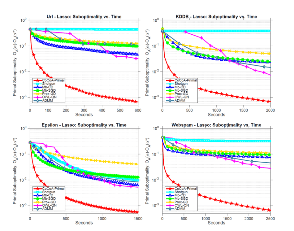
clearly, CoCoA converges 50x faster than the best competing method OWL-QN, performing most remarkably on datasets with large number of features, which are exactly the cases where lasso is often applied.
In the dual setting, we consider fitting an SVM. CoCoA uses stochastic dual coordinate ascent as local solver. All methods distribute datasets by data points. Evidently, CoCoA is able to outperform all other methods with a large margin.

To understand the primal-dual interchangeability of CoCoA, we fit an elastic net regression model for both variants, with coordinate descent as local solver.

Primal CoCoA performs better on datasets with a large number of features relative to data points, and is robust to deterioration in strong convexity. On the other hand, dual CoCoA shines when datasets have large number of points relative to features, and is subpar in terms of robustness against loss of strong convexity. This prompts practitioners to use different CoCoA variants, Algorithm 2 or Algorithm 3, for different problem settings.
More interesting findings are reported in the original paper, for example primal CoCoA preserves local sparsity and translates it into global sparsity, tuning H as proxy of ![]() allows ML system designers to navigate along the computation-communication tradeoff curve and strike the best balance for their system at hand.
allows ML system designers to navigate along the computation-communication tradeoff curve and strike the best balance for their system at hand.
Conclusion
CoCoA is a general-purpose distributed optimization framework that enables communication-efficient primal-dual optimization in a distributed cluster, by leveraging duality to decompose the global objective into local quadratic approximate subproblems, which can be solved in parallel to arbitrary accuracy by any state-of-the-art single-machine solver of the architect’s choice. CoCoA’s flexibility allows ML system designers and algorithm authors to easily navigate along the computation-communication tradeoff curve of a distributed system, and choose the optimal balance for their particular hardware configuration and computation workload. In the experiments, CoCoA summarizes this choice into a single tunable hyperparameter H (number of total iterations), whose equivalent ![]() (local solution quality) factors into two important theoretical proofs of the convergence rates for primal and dual CoCoA. Empirical results show CoCoA is able to outperform state-of-the-art distributed optimization methods by margins as large as 50x.
(local solution quality) factors into two important theoretical proofs of the convergence rates for primal and dual CoCoA. Empirical results show CoCoA is able to outperform state-of-the-art distributed optimization methods by margins as large as 50x.
References
[1] CoCoA: A General Framework for Communication-Efficient Distributed Optimization, V. Smith, S. Forte, C. Ma, M. Takac, M. I. Jordan, M. Jaggi, https://arxiv.org/abs/1611.02189
[2] Distributed Optimization with Arbitrary Local Solvers, C. Ma, J. Konecny, M. Jaggi, V. Smith, M. I. Jordan, P. Richtarik, M. Takac, Optimization Methods and Software, 2017, http://www.tandfonline.com/doi/full/10.1080/10556788.2016.1278445
[3] Adding vs. Averaging in Distributed Primal-Dual Optimization, C. Ma*, V. Smith*, M. Jaggi, M. I. Jordan, P. Richtarik, M. Takac, International Conference on Machine Learning (ICML ’15), http://proceedings.mlr.press/v37/mab15.pdf
[4] Communication-Efficient Distributed Dual Coordinate Ascent, M. Jaggi*, V. Smith*, M. Takac, J. Terhorst, S. Krishnan, T. Hofmann, M. I. Jordan, Neural Information Processing Systems (NIPS ’14), https://people.eecs.berkeley.edu/~vsmith/docs/cocoa.pdf
[5] L1-Regularized Distributed Optimization: A Communication-Efficient Primal-Dual Framework, V. Smith, S. Forte, M. I. Jordan, M. Jaggi, ML Systems Workshop at International Conference on Machine Learning (ICML ’16), http://arxiv.org/abs/1512.04011
Author: Yanchen Wang
0 comments on “System-Aware Distributed Optimization for Machine Learning”